
Wading through Graph Neural Networks
- Topics
- Graph and its motivation
- Graph Convolutional Networks
- Graph Attention Networks
- Gated Graph Neural Networks
- Graph AutoEncoders
- Graph SAGE
- Some history behind GCNs
- Conclusion
- References
In this blog, I am going to discuss Graph Neural Network and its variants. Let us start with what graph neural networks are and what are the areas in which it can be applied. The sequence in which we proceed further is as follows:
Topics
- Graph and its motivation
- Graph Convolutions
- Graph Attention Networks
- Gated Graph Neural Networks
- Graph AutoEncoders
- Graph SAGE
- History behind GCN
Graph and its motivation
As the deep learning era has progressed so far, we have many states of the art solutions for datasets like text, images, videos etc. Mostly those algorithms consist of MLPs, RNNs, CNNs, Transformers, etc., which work outstandingly on the previously mentioned datasets. However, we may also come across some unstructured datasets like the ones shown below:

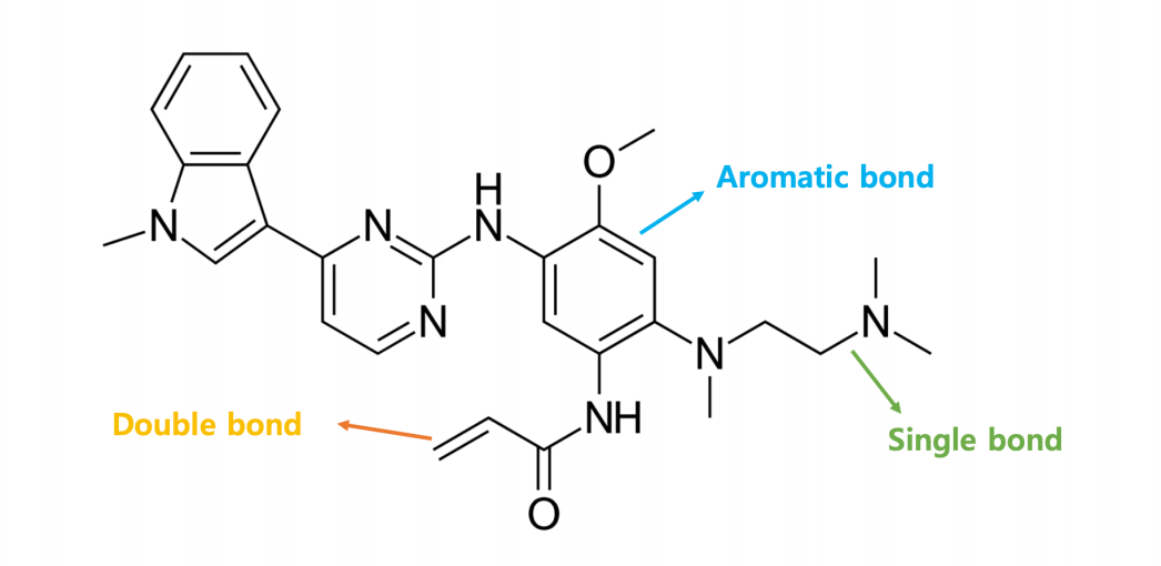
All you need to represent these systems are graphs and that is what we are going to discuss further. Lets us briefly understand how a graph looks like: A graph G is represented by two key elements, {V, E} where V is the set of nodes and E is the set of edges defined among its nodes. A graph neural network has node features and edge features where node features represent the attributes of individual elements of a system and the edge features represent the relationship, interaction or connectivity amongst the elements of the system.
Node features:
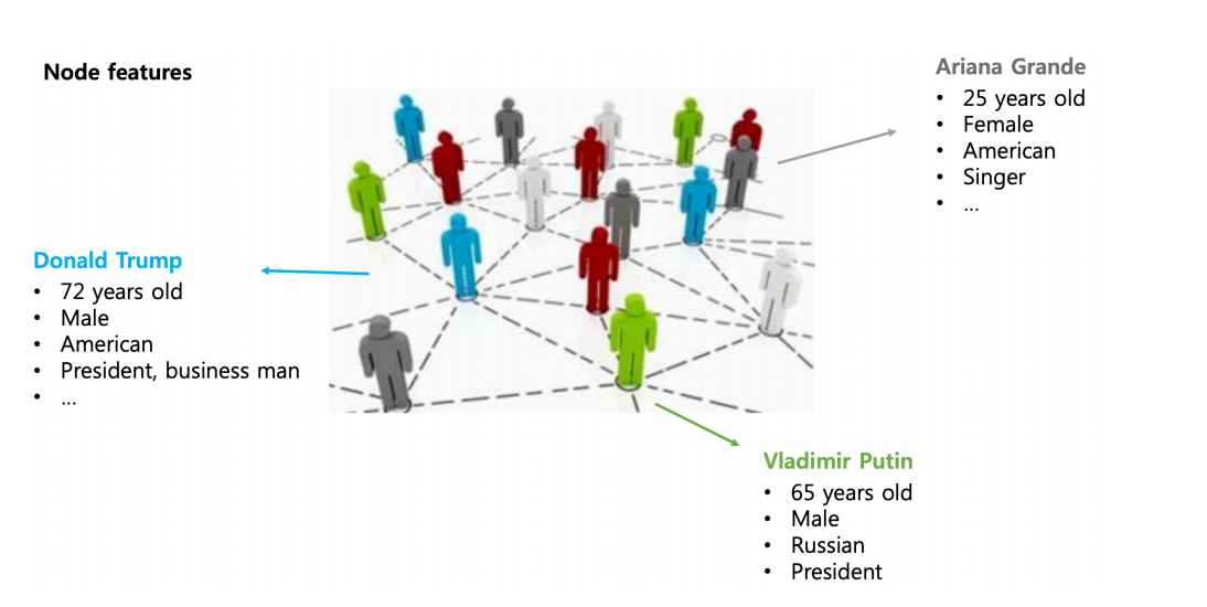
Edge features:
A graph neural network can learn the inductive biases present in the system by not only producing the features of the elements of a system but understanding the interactions among them as well. The capability of learning of the inductive biases from a system makes it suitable for problems like few-shot learning, self-supervised or zero-shot learning. We can use GNNs for purposes like node prediction, link prediction, finding embeddings for node, subgraph or graph etc. Now let us talk about graph convolutions.
Graph Convolutional Networks
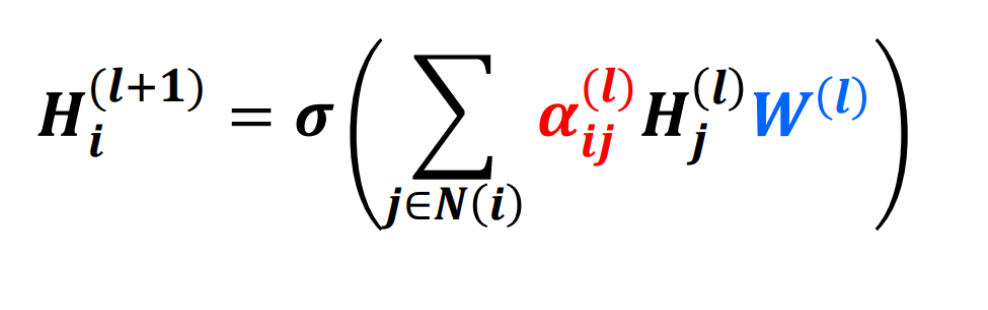
So in a graph problem, we are given a graph G(V, E) and the goal is to learn the node and edge representations. For each vertex i, we need to have a feature vector Vᵢ and the relationship between nodes can be represented using an adjacency matrix A. GCN can be represented using a simple neural network whose mathematical representation is as follows:

where Hᵢˡ is the feature vector of node i in the lᵗʰ layer, Wˡ is the weight matrix used for the lᵗʰ layer and N(i) is the set of nodes in the neighbourhood of node i. Note that Hᵢ⁰=Vᵢ Now as you can see the weights are shared for all the nodes in a given layer akin to conventional convolutional filters and the feature vector of a node is computed upon performing some mathematical operation(here weighted sum using the edge parameter) on its neighbourhood nodes(which also is similar to that of a CNN), we come up with the term Graph Convolutional Network and Wˡ can be called as a filter in layer l. As it is evident, we see two issues here, the first being that while computing the feature vector for a node, we do not consider its own feature vector unless a self-loop is there. Secondly, the adjacency matrix used here is not a normalised one, so it can cause scaling problem or gradient explosion due to the large values of the edge parameters. To solve the first issue a self-loop is enforced and to solve the second one, a normalized form of the adjacency matrix is used which is shown below:
- Self-Loop: Â =A+I
- Normalization: Â = (D^(-1/2))Â(D^(-1/2))
where I is an identity matrix of shape A and D is a diagonal matrix whose each diagonal value correspond to the degree of the respective node in matrix Â. In each layer, the information is passed to a node from its neighbourhood, thus the process is called Message Passing. Now let us talk about some variants of the simple graph convolution we just talked about.
Graph Attention Networks
Attention is not a new thing in the tech world. It has been widely used with architectures like LSTMs, GRUs, CNNs, etc. Now, it is even capable of being the sole and most important building block of transformers based models like BERT and GPT. So, the main purpose of attention mechanism is to focus on some key areas of the input by learning weights for them in the form of probabilities. Lets us see briefly how it works when it is used in a graph neural network.
Given above, is a modified equation for a graph convolution. The difference being the term:
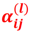
These are nothing but the attention weights. For each neighbour node j of node i in the lᵗʰ layer, a weight is learned which denotes its importance while updating the feature vector of node i. Therefore instead of finding a simple weighted sum of the neighbours, we take more information from the nodes whose attention weights are more and less information from the lesser weighted nodes. Now, these weights can be learned in various ways such as softmax or some squash functions as shown below:
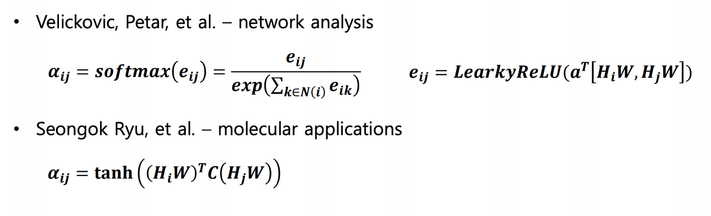
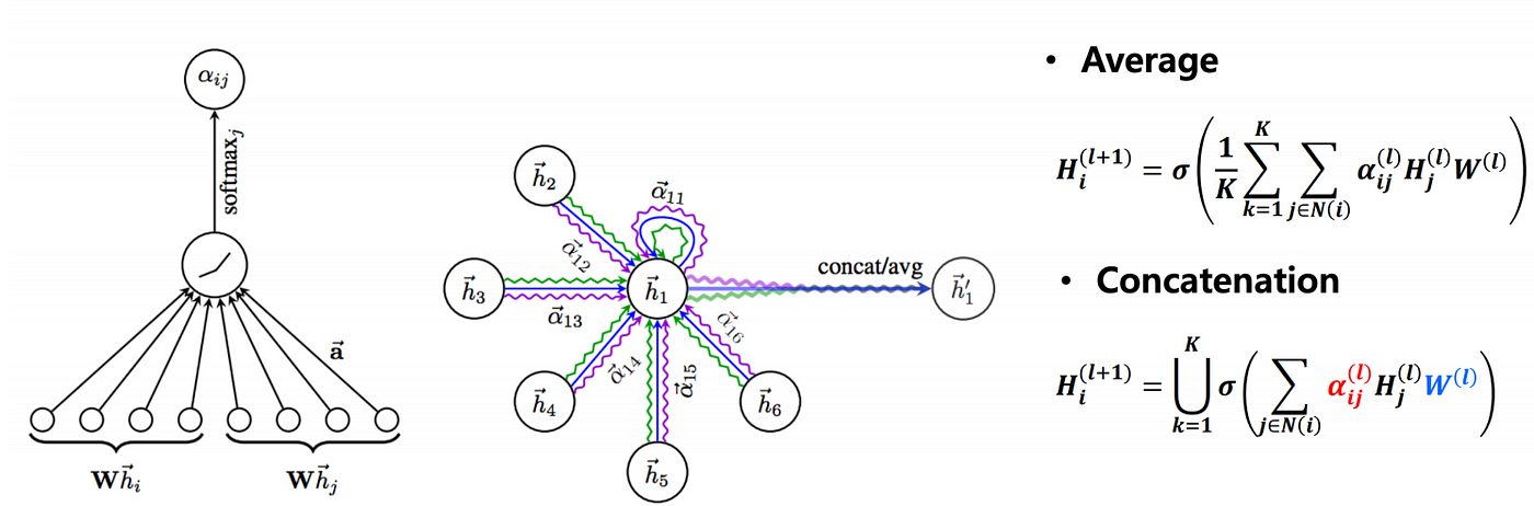
To make things more interesting, we can use the multi-head attention approach also which will use K heads instead of one and finally take the average(or concatenate) of all the feature vectors learned from the K heads. An illustration can be found in the figure given below:
Gated Graph Neural Networks
Now suppose we want to build a model for a sequential dataset like texts but each element in the sequence can not be just represented through an embedding like Glove and is taking the form of a graph-like structure. This is the time my friends, we need to discuss gated graph neural networks. These networks can be used to work around sequential graphs. So, basically each node is updated using the previous node state and the current message state like GRU. Node states and message states are similar to that of hidden states and cell state in an RNN cell. The formula below explains the theory clearly:
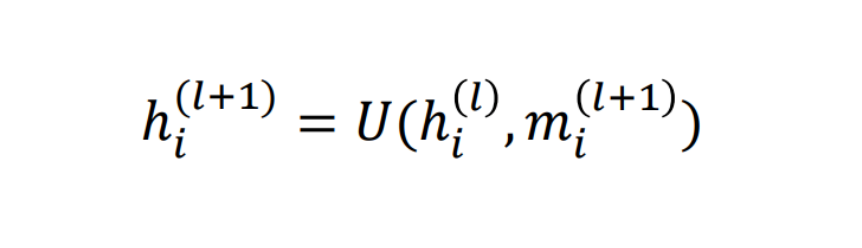
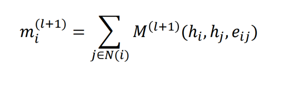
In the given equations, hˡᵢ is the node state of node i in layer l and mˡᵢ is the message state of node i in layer l. U and M can be understood as vanilla neural networks.
Graph AutoEncoders
Similar to other autoencoders, we can have a graph autoencoder too. Graph autoencoders can be useful for node-compression or self-supervised training of graph data structures. In this, we first find a latent feature vector representation for the nodes in the graph and then learn to reconstruct the original adjacency matrix from the latent representation. Again, to complicate things, we can use variational graph autoencoders. A graph autoencoder looks like the one shown in the figure below:
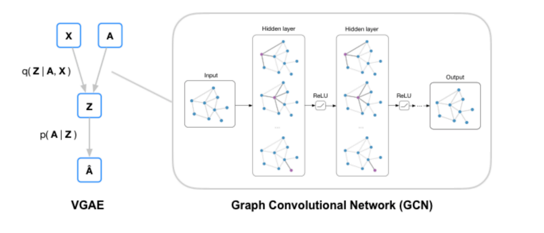
| Given a graph G(X, A), we learn the latent representation of the nodes by learning the distribution q(z | X, A). And then we try to reconstruct the adjacency matrix Â, by learning the distribution p(A | Z). |
Graph SAGE
Ever thought of the fact that we aggregate the neighbourhood information of a node by taking the weighted average of the features of its neighbour nodes in a typical GCN. The question is can we try something more or better. This is where we discuss Graph SAGE. In this, instead of taking a weighted average of the neighbour nodes, we try to learn a function approximator which aggregates the information of the neighbourhood of a node when its feature vector is being updated. The figure below will make it understand clearly:
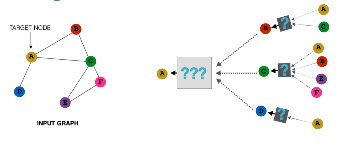
The black box given in the figure above is a differentiable function which takes some vectors as inputs, aggregates their information into a single feature vector. The equation for the same is as follows:

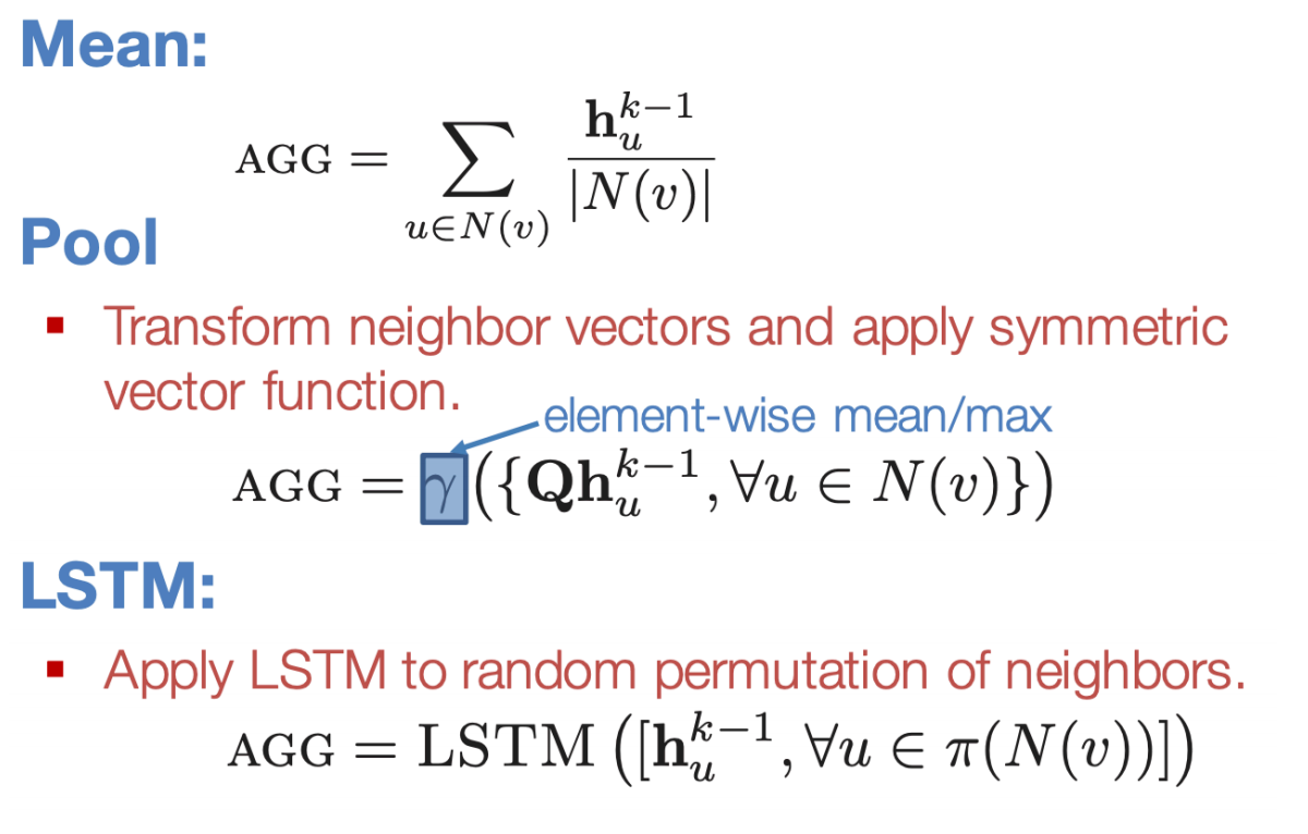
where hᵥᵏ is the feature vector of node v in the layer k, A and B are trainable weights. The aggregated neighbourhood information and the node feature vector itself are concatenated by performing some weighting and then fed through a non-linear function σ to get the node feature vector for the next layer. AGG is the aggregator function and can have many forms like mean, pool or LSTM aggregator as shown below:
Some history behind GCNs
The methods we discussed above were all using spatial filters but we have another type of filters in graph neural networks too, SPECTRAL FILTERS. Using spectral filters requires us to go into the spectral domain(Fourier domain) which further requires us to compute the eigenvector decomposition of the graph Laplacian L which is a special normalised form of the adjacency matrix of a graph G. L = I —  where  is the normalised adjacency matrix discussed at the start of the blog and I is the identity matrix. L is decomposed into the form, L=VΛVᵀ where V is the matrix of eigenvectors of L and Λ is a diagonal matrix whose diagonal values correspond to the eigenvalue of L. The equation for the forward-pass is given below:
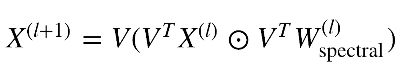
where W is the weight matrix and the dot is element-wise multiplication. For large adjacency matrices, it becomes an unfeasible task to compute the decomposition thus making the process computationally very expensive. Chebyshev graph convolution approximation introduced by Defferrard et al., NeurIPS, 2016, prevented the decomposition of laplacian by using Chebyshev approximation and introducing a parameter K. For K=1, we pass the node features X⁽ˡ⁾ in our GNN model; for K=2, we pass X⁽ˡ⁾, AX⁽ˡ⁾ ; for K=3, we pass X⁽ˡ⁾, AX⁽ˡ⁾, A²X⁽ˡ⁾ and similarly for K=n, we pass X⁽ˡ⁾, AX⁽ˡ⁾, A²X⁽ˡ⁾……..AⁿX⁽ˡ⁾ in the GNN model. Once all the features from the n hops are created, we concatenate all the feature vectors and then again a GNN is applied to get the final feature vectors for the nodes. The process gets clear from the image given below:
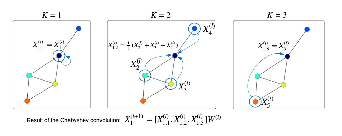
Chebyshev approximation does get rid of the spectral domain but still, it is computationally expensive because of the iterative n(decided by us) hops in a single layer.
Further approximation and Renormalization Trick
Since increasing the value of K leads to an increase in number of parameters of the model, we can restrict the value to K=2.
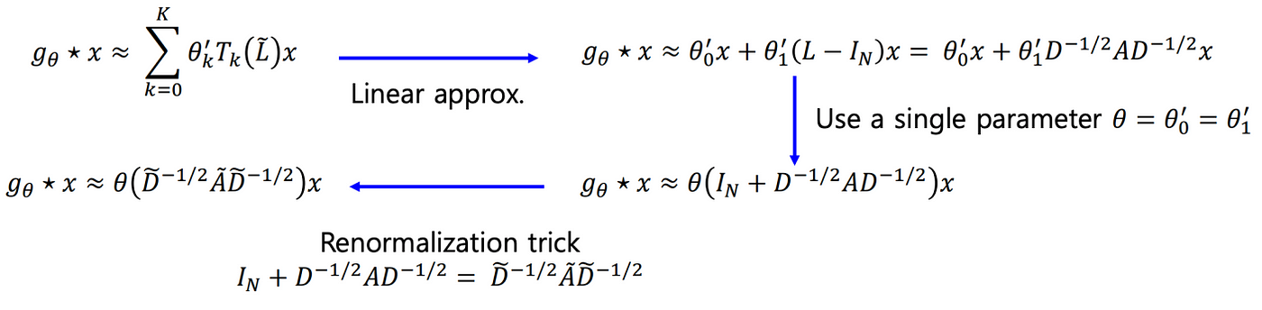
The A used in the above illustration is the original adjacency matrix without self-loop enforcement. By using a trick or say approximation of assigning the same θ for θ₀ and θ₁ leads us to a renormalization trick which we already had discussed in the GCN part(adding self-loop). Thus the approximation gives us our GCN layer which works for 1 and 2 hops and if we want more than 2 hops we can keep adding such GCN layers.
Conclusion
So far we discussed the motivation behind using graph neural networks origination of GCNs and their variants. In the next blog, I intend to discuss some cool applications of GCNs like text classification, link prediction, zero-shot sketch-based image retrieval and many more.