In the previous blog, we dived into the basic implementation of a deep Q-Learning Neural Network. It was a Policy-based duel- network which was used to learn the thief-police-gold game. Now, I have all of a sudden introduced two terms here, Policy-Based, Duel-Network. Policy-based methods are those which learns the probability distribution of the actions to take next of being in a given state. As, it could be seen that we were using a softmax layer of output-size=number of possible actions, it was nothing but the policy-learning mechanism for the network to learn which action to take further depending on the probabilities. Moving on to the next term, Duel-Network. We had used two neural-networks in the previous blog, one which was used and updated in an online manner while the other was updated(not so often) and used for predicting the policy values for the new_state. The reason for that was to be able to maintain some sort of consistency and not induce much randomness in the poilcy-prediction for the new states which are used to update the current policy-values.

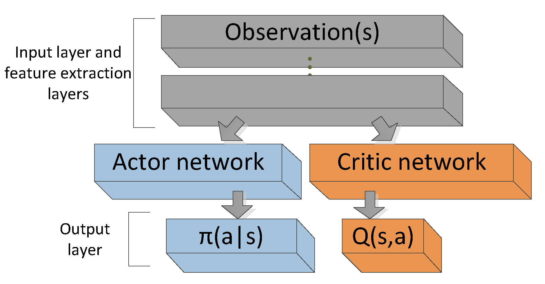
Coming to this blog, I will be talking about a new term again 😀 and that is Actor-Critic Methods. The previous agent can be understood as the actor part of the actor-critic networks as it focuses on the policy-prediction. To be able to understand the critic part, we need to understand value-based networks. So, unlike policy based networks critic-network predicts the value of importance of being in a state(state-value) or for a action-state pair(q-value). In fact, reinforcement learning started with value-based networks only and the policy-based learning was further derived using the equation of value-equation.

Let us go into some maths this time 😊:

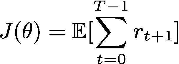
The main aim of a reinforcement learning algorithm is to maximise the reward considering the future actions and their rewards. Mathematically this can be shown as :

Now that we have talked about the policy function earlier in this post, let us look into the mathematical expression of the gradients of the cost function J(θ) required for updating the policy functions. We call them policy gradients. A very nice derivation of getting the gradients is given in this blog. If you feel curious, you can read it. So, the final expression for the gradient is as follows:

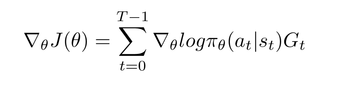
where G the sum of future discounted rewards:

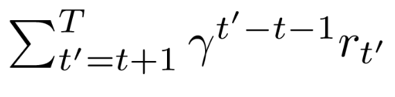
So, G is nothing but the Q-value. Hence, we can now approximate both actor(softmax) and critic(logits) by using a single neural network. But further research suggested a slight improvement in the expression and instead of using G, an Advantage Function is used which is defined as follows:

where, V is the state-value function. We can still use a single neural network to approximate both the critic and the actor, thanks to the bellman optimal equation which gives a direct mapping between the Q value and the state-Value functions. As a result, we can directly replace the G with the advantage function, A in the policy gradient equation.

This results in naming the algorithm to Advantage Actor Critic(A2C), where there is only one agent having two networks, actor and critic parametrised by a single neural networks whose weights are updated using Advantage Value and the cross-entropy loss. We will cover the loss calculation part too in this blog. But before that, I will discuss about one more famous algorithm proposed by DeepMind which is an extended version of the A2C.

A3C Algorithm

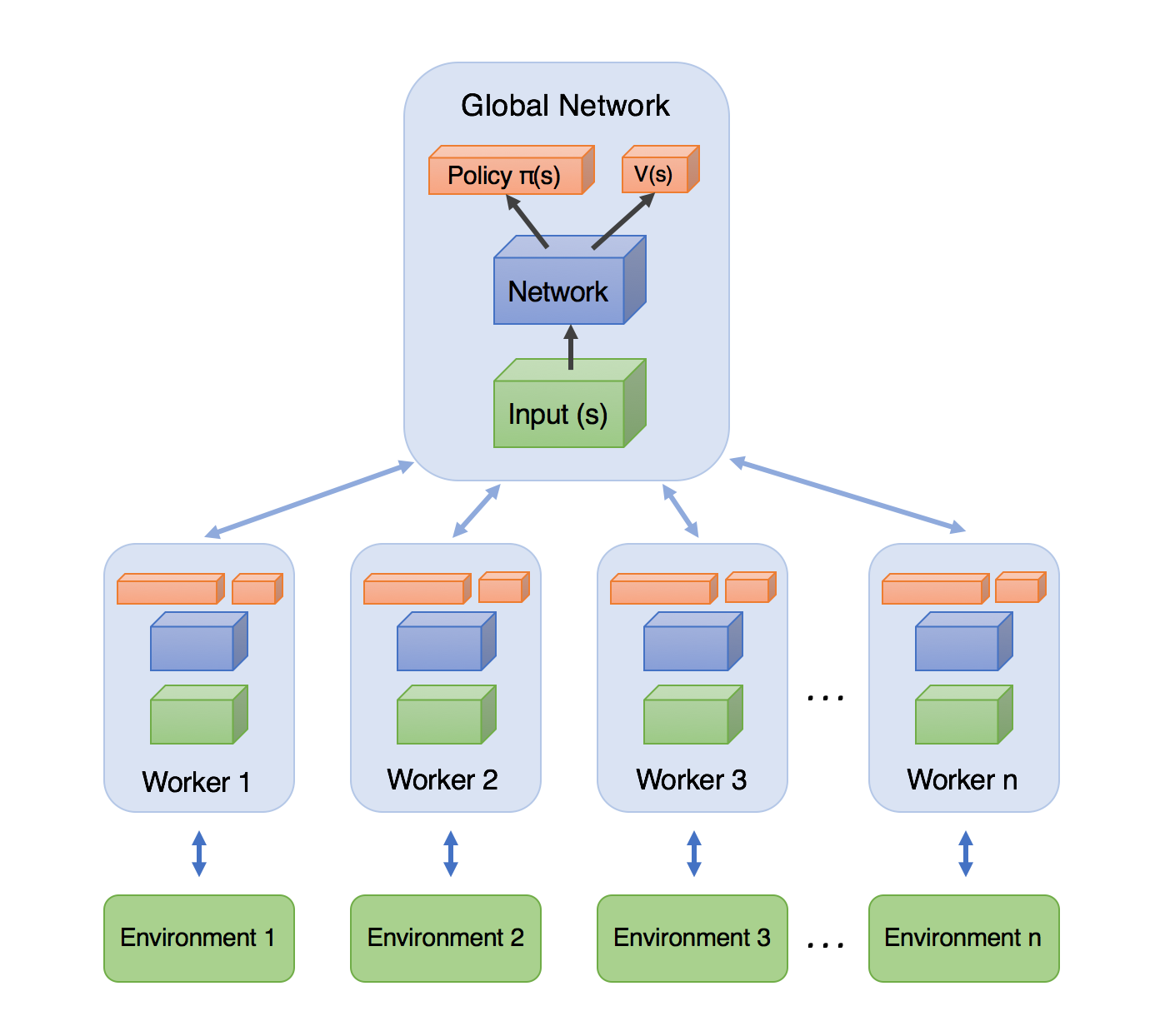
So the extra A which gets added in this algorithm, comes from the term, Asynchronous. In this method, there is a global network with shared parameters just like the predict_model in the previous blog. Apart from that there are multiple agents exploring the environment, instead of only a single agent. All those agents learn independently as each of them have their own copy of the environment. The term asynchronous comes here as they learn and update the global network asynchronously. Meaning, each of them explore the environment parallelly and while one of them is updating the global network, the other wait and update the global network when their turn comes.

Results, show that despite of the size and complex nature of A3C, A2C manages to perform somewhat closer to it but still, A3C turns out to be more consistent because of the multi-agent exploration strategy.

Now let us discuss the loss part:

1.Critic Loss : This will be computed as the mean squared loss which can be shown as follows:

CLoss = Σ(R-V)^2,

where R is the discounted sum of future rewards in the trajectory.

2. Actor Loss : This is computed first by taking the categorical-cross entropy taking the label as the action taken randomly and multiplying that value with the advantage value, (R-V).

I will soon be adding the code for the A2C and A3C networks in this blog. Hope you liked it.

Keep Learning, Keep Sharing