BiDirectional Attention Flow Model for Machine Comprehension
- Highway Networks
- Similarity Matrix
- Context2Query and Query2Context Attention
- Merge Operation
- Similarity Matrix
- Context2Query Attention
- Query2Context
- The MegaMerge
- The Highway LSTMs
- Results and Conclusion
- References
- Keep Learning, Keep Sharing 🤟
Question Answering has been a major area of work in Natural Language Processing. I will be discussing as well as implementing the key elements of a research paper which does significantly well on QA related problems. So, What do we do in Question Answering? We are given a context and a query is asked based on that context. The task of the model is to find an accurate answer to the problem. The answer may or may not be present in the context itself. If it is present, the task can be formulated as a classification problem and if it is not present, then we move to a much tougher text-generation problem. But for all of that we need a fine feature vector which contains the information from context and query and their relationship.
The paper which I will be talking about is Bidirectional Attention Flow For Machine Comprehension by Minjoon Seo et al. We will be discussing mainly the technical segments of the architecture and will be implementing those sections sequentially. Overall, it will mostly be code writing with lesser text here. Given below is the architecture of BiDAF.
As given in the figure, the text representation in the model is done by first using a character level embedding layer and then word level embeddings like Glove or Word2vec. Finally both the representations are concatenated together to get the final representation. For simplicity, we can only use word-level Glove Embeddings in the code.
Once we get the vector representation for each word in the text sequence, we will feed the sequence in a bidirectional LSTM layer to get fine contextual representations. One important thing which is not shown in the figure is the Highway Networks. Since, I have not mentioned this term in any of my previous blogs, we will discuss it briefly before moving to the implementation part.
Highway Networks
Imagine a network having very deep structure including multiple stacks of NN Layers. Earlier experiments suggest that optimizing a model with depth greater than 19 was harder with gradient descent. Also, if multiple stacks are used information loss is observed because of multiplication of too many variables having absolute values less than 1. Thus, increasing depth of the model beyond a certain point did not benefit the results earlier.
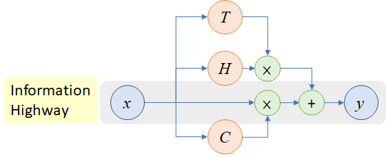
Inspired by LSTMs, Highway Networks were proposed in which a gating mechanism is used to propagate information directly to the next layers(thus the term HIGHWAY). The structure for the same is shown below:

A transform gate, T is introduced which is nothing but a neural network followed by a sigmoid activation. It means the transform gate will produce a probability which gets multiplied with the output of the current layer and is propagated to the next layer. The linear gate, C is nothing but 1-T, which is the probability to be multiplied with the input of the current layer and passed in the next layer. A variant of Highway Networks, Residual Networks where C and T both are equal to 1, is used in the famous image classification model by Microsoft, ResNet. Results show that it is now possible to have a model with 100s of layers using Highway Networks for complex problems.
In this blog, we will also be using Highway Networks for each bidirectional LSTM to have a robust information flow.
Similarity Matrix
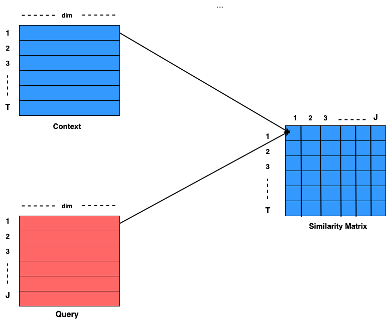
Normally, Attention Mechanism is used to summarize the context vector for the query. But here, a shared Similarity Matrix is computed by using the context and query representation and instead of computing a single attention for the query, Attention in both direction, i.e., Context2Query and Query2Context is computed for maximizing the information gain. Similarity Matrix is a matrix of shape TxJ where T is the sequence length of Context and J is the sequence length of Query. Both the attentions can be computed by the shared Similarity Matrix. The entire computing mechanism is shown in the figure below:

It can be seen that to compute Sij, input is Ci and Qj and the formula for that is as follows:
F(Ci, Qj) = Wij[ Ci ; Qj ; Ci o Qj],
where [;] is the concatenation operation across row and [o] is element wise multiplication operation and Wij is a trainable weight vector of size [1 x 3 * dim].
Context2Query and Query2Context Attention
Context2Query Attention signifies the important words in the query sentence for each context word. That means the Context2Query should be of shape, [TxJ] which can be done just by taking the softmax of similarity Matrix row-wise:
C2Q = Softmax(S, axis=-1)
Attended Query, AQ = C2Q.Query, shape=[Txdim], [. = Matrix Multiplication]
Query2Context Attention signifies the most similar words in the context sentence for each query word. This is obtained by first taking maximum element from the Similarity matrix and then applying softmax on it. Thus the final output is a probability vector of shape = [Tx1].
Attended Context = Q2CTContext, shape=[1xdim]
The final Attented Context, AC = tile(Attended Context, T), shape = [Txdim]
Merge Operation
This operation is used to combine the information obtained by the attentions C2Q and Q2C. The merge operation takes the original context(OC), attented query and attented context as inputs and gives a final representation as shown below:
Merge(OC, AQ, AC) = [OC ; AQ ; OC o AQ ; OC o AC] , where [;] is row-wise concatenation and [o] is element wise multiplication.
Merger Layer gives us an output of shape = [T x 4 * dim], which can be further used to fed into another set of bidirectional LSTMs followed by a softmax to get the start and end probabilities of the answer. The start and end probabilities are the probabiltities of start and end index of the answer in the given paragraph. As earlier discussed, the concept of start and end probabilities will work only if the answer lies within the paragraph. If it does not, we have feed the final representation to a decoder to make it a sequence generation problem.
Whoo ! I did not keep my promise of keeping the discussion short and sticking mainly to the coding part 😀. Anyways, let us do some PYTHONING now(Google’s Meena told me about this word).
Similarity Matrix
class SimilarityMatrix(keras.layers.Layer):

    def __init__(self,dims, **kwargs):
        self.dims = dims
        super(SimilarityMatrix, self).__init__(**kwargs)

    def similarity(self, context, query):
        e = context*query
        c = K.concatenate([context, query, e], axis=-1)
        dot = K.squeeze(K.dot(c, self.W), axis=-1)
        return keras.activations.linear(dot + self.b)

    def build(self, input_shape):
        dimension = 3*self.dims
        self.W = self.add_weight(name='Weights',
                                shape=(dimension,1),
                                initializer='uniform',
                                trainable=True)

        self.b = self.add_weight(name='Biases',
                                shape=(),
                                initializer='ones',
                                trainable =True)

        super(SimilarityMatrix, self).build(input_shape)

    def call(self, inputs):
        C, Q = inputs
        C_len = K.shape(C)[1]
        Q_len = K.shape(Q)[1]
        C_rep = K.concatenate([[1,1],[Q_len],[1]], 0)
        Q_rep = K.concatenate([[1],[C_len],[1,1]],0)
        C_repv = K.tile(K.expand_dims(C, axis=2),C_rep)
        Q_repv = K.tile(K.expand_dims(Q, axis=1), Q_rep)

        return self.similarity(C_repv, Q_repv)

    def compute_output_shape(self, input_shape):
        batch_size = input_shape[0][0]
        C_len = input_shape[0][1]
        Q_len = input_shape[1][1]
        return (batch_size, C_len, Q_len)

    def get_config(self):
        cofig = super().get_config()
        return config
Context2Query Attention
class Context2QueryAttention(keras.layers.Layer):
    def __init__(self, **kwargs):
        super(Context2QueryAttention, self).__init__(**kwargs)


    def build(self, input_shape):
        super(Context2QueryAttention, self).build(input_shape)

    def call(self, inputs):
        mat,query = inputs
        attention = keras.layers.Softmax()(mat)
        return K.sum(K.dot(attention, query), -2)

    def compute_output_shape(self,input_shape):
        mat_shape, query_shape = input_shape
        return K.concatenate([mat_shape[:-1],query_shape[-1:]])

    def get_config(self):
        config = super().get_config()
        return config
Query2Context
class Query2ContextAttention(keras.layers.Layer):
    def __init__(self, **kwargs):
        super(Query2ContextAttention, self).__init__(**kwargs)


    def build(self, input_shape):
        super(Query2ContextAttention, self).build(input_shape)

    def call(self, inputs):
        mat,context = inputs
        attention = keras.layers.Softmax()(K.max(mat, axis=-1))
        prot = K.expand_dims(K.sum(K.dot(attention,context),-2),1)
        final = K.tile(prot, [1,K.shape(mat)[1],1])
        return final

    def compute_output_shape(self,input_shape):
        mat_shape, cont_shape = input_shape
        return K.concatenate([mat_shape[:-1],cont_shape[-1:]])

    def get_config(self):
        config = super().get_config()
        return config
The MegaMerge
 class MegaMerge(keras.layers.Layer):
    def __init__(self, **kwargs):
        super(MegaMerge, self).__init__(**kwargs)

    def build(self, input_shape):
        super(MegaMerge, self).build(input_shape)

    def call(self, inputs):
        context, C2Q, Q2C = inputs
        CC2Q = context*C2Q
        CQ2C = context*Q2C
        final = K.concatenate([context, C2Q, CC2Q, CQ2C], axis=-1)
        return final

    def compute_output_shape(self, input_shape):
        C_shape,_,_ = input_shape
        return K.concatenate([C_shape[:-1], 4*C_shape[-1:]])

    def get_config(self):
        config = super().get_config()
        return config
The Highway LSTMs
class HighwayLSTMs(keras.layers.Layer):
    def __init__(self, dims, **kwargs):
        self.dims = dims
        super(HighwayLSTMs, self).__init__(**kwargs)

    def build(self, input_shape):
        self.LSTM = keras.layers.Bidirectional(keras.layers.LSTM(self.dims, return_sequences=True))
        super(HighwayLSTMs, self).build(input_shape)

    def call(self, inputs):
        h = self.LSTM(inputs)
        flat_inp = keras.layers.Flatten()(inputs)
        trans_prob = keras.layers.Dense(1, activation='softmax')(flat_inp)
        trans_prob = K.tile(trans_prob, [1,2*self.dims])
        trans_prob = keras.layers.RepeatVector(K.shape(inputs)[-2])(trans_prob)
        out = h + trans_prob*inputs
        return out

    def compute_output_shape(self, input_shape):
        return input_shape

    def get_config(self):
        config = super().get_config()
        return config
The only thing remains now is to apply these snippets into one’s use case. I hope I did not bore you(definitely not, if you are reading this line).
Results and Conclusion
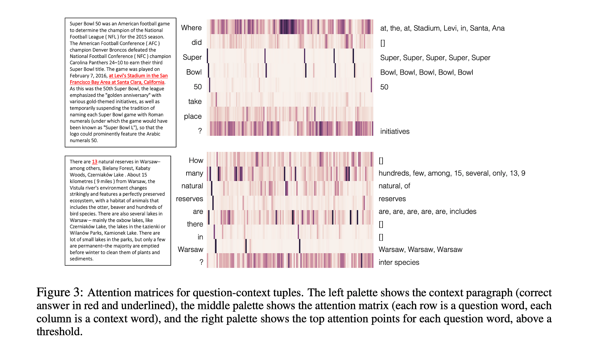
We have now discussed the technical aspects and implementation of various sections of a BiDAF model. Now, let us wade through an example of how this attention mechanism comes up with the answers for a particular question.

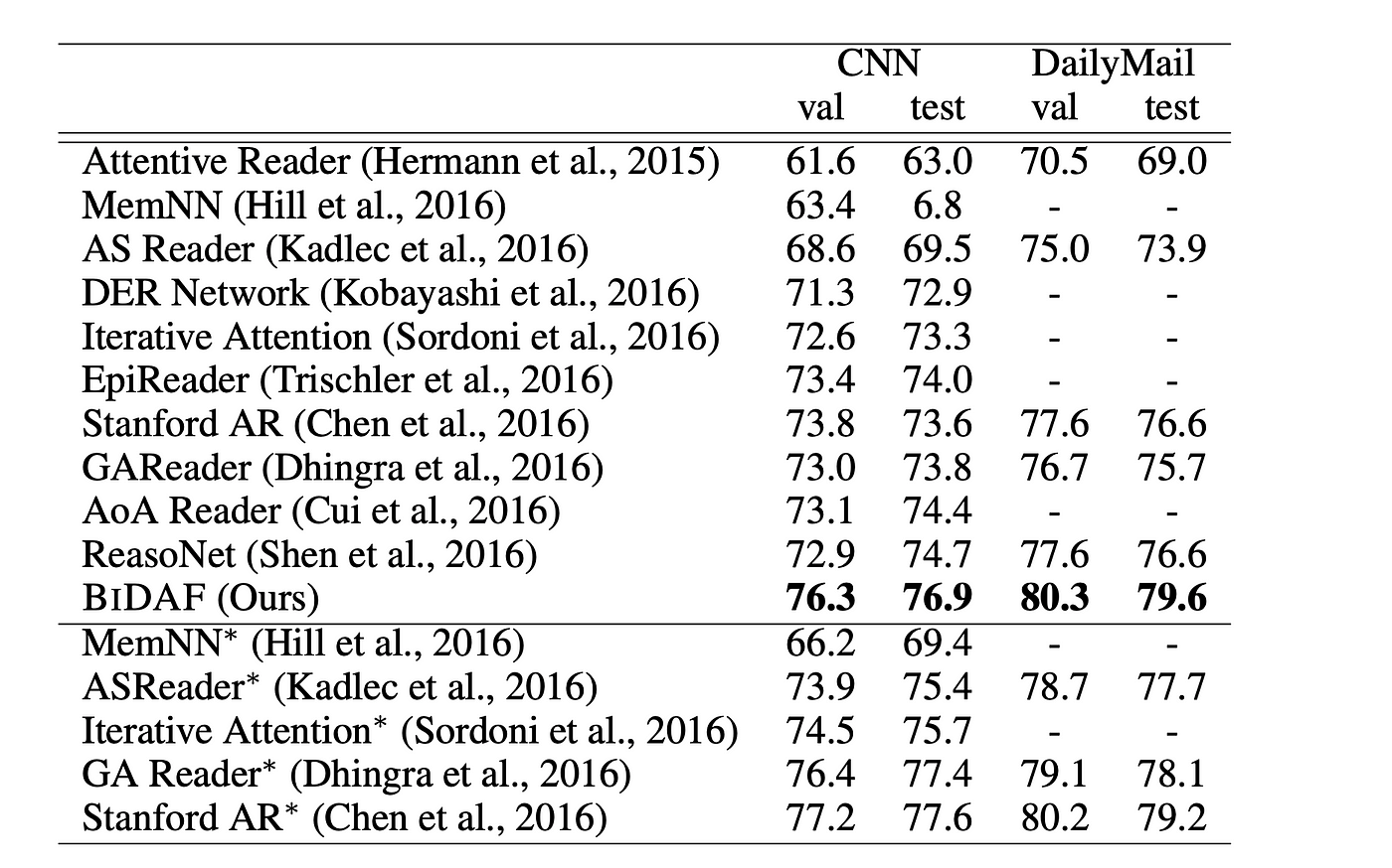
In the image shown above, the blocks given is the attention matrix visualisation of two questions. Each column of the matrix denotes the context words in the paragraph while each row represents the words in the question vector. The bolder the block, the more its attention weights are. In the block 1, it is clearly visible that for the word, “Where” in the question, more weights are given to the words, “at, the, stadium, Levi, in, Santa, Ana”. Even it can focus on the question mark, ‘?’ which attends more on the “initiatives” word. From the results perspective, BiDAF was tested against SQUAD, CNN/DailyMail datasets and the results were outstanding as follows:

References
If you wish to read more about the topics, there is nothing better than the research papers themselves.
- BiDAF: https://arxiv.org/pdf/1611.01603.pdf
- Highway Networks: https://arxiv.org/abs/1505.00387
I hope you liked the blog and if you have any suggestions for me or you feel like connecting, you can click on the links below:
Linkedin: https://www.linkedin.com/in/spraphul555/
Time for the signature Line,

